A Working List of Probability Questions: Week 2

Market Making, Expected Value, and General Topics
June 28, 2020 | Updated July 6, 2020

Welcome to week two of my trading prep series! This week I’m going to focus most of my attention on learning and practicing market making, expected value, and other expanded topics. I’ll also post resources and links to additional problems as I go along for my documentation purposes. Thanks for tuning in!

Update: Instead of doing $5$ problems every day consecutively, I’ll be doing problems on weekdays and spending weekends reviewing problems and topics I’ve already covered.

Day Eight: June 29

A friend linked me to a blog post by Messy Matters on confidence intervals/overconfidence that you can find here. I’ve been spending some time with market making questions so I found the excercise and results of the “study” pretty interesting. I also found this powerpoint on recuiting tips when I was looking for new problems to do.

Problem 1. Make me a market on the temperature in an hour. Solution. I was thinking through this problem after taking a walk this morning. At the time, I estimated the temperature to be about $60^\circ - 65^\circ$ (the actual temperature was $64^\circ$). Given it was $10\colon 35AM$, it’s still relatively early in the day and there’s quite a bit of room for the temperature to increase to before it plateaus in the afternoon. From my experience, the temperature in a typical summer day in San Francisco usually tops off around $75^\circ$ to $85^\circ$. This morning was relatively cool and so I’d expect that today would be one of the cooler days, toping off between $75^\circ$ to $78 ^\circ$. Then, just assuming that the temperature increases somewhat linearly, I’d set my bid at $63^\circ$ and offer at $68^\circ$.

After setting my initial spread, I’d adjust my interval accordingly to how the second party/market makers chooses to buy from or sell to me. To do this, I sampled from a normal distribution meaned at $65.5$ with $\sigma = 0.83$ for the price and flipped a coin to determine whether I was being bought or sold to at that price.

1. Bid at $66.9^\circ$: buying from me at a value leaning so far to the right in my range indicates that I severely underestimated the temperature in an hour, as the willingness to buy higher might be an attempt to execute an unfavorable trade with me to then later sell at a higher price with an acceptable margin. However, I also know the temperature cannot change too much so I’d adjust my spread to account for this new information by shifting my position to $65.5-71$. I widened my range a bit since I’m pretty skeptical that my original range reflected the actual temperature well and I want to make sure to cover all my bases.
2. Offer at $68.4^\circ$: A willingness to sell indicates that, taking into account my decision-making, the second party believes that $68.4^\circ$ optimizes both margins and chance of trade execution. I wouldn’t expect the exact temperature to be $68.4^\circ$ since not all buyers with information on the weather would want to buy the exact of the instrument as it’s harder to later sell for profit. I’d adjust my spread down to $66.5 - 69.5$.

Unfortunately, this simulation is flawed as I didn’t really have a second party with better information on the specific product being exchanged. I tried to adjust for that by using the sampler and randomizing but since the real value of the temperature at $11\colon35$ wasn’t known to either me or my fictitious party, I had to operate under the assumption that my initial spread wasn’t completely wrong, which could have been the case. Next time, I’ll probably try this with a partner. The actual temperature at $11:35$ was about $66^\circ$ so you can see how the spread deviated from that without this information, but this exercise still helps me practice adjusting my spread to new information.

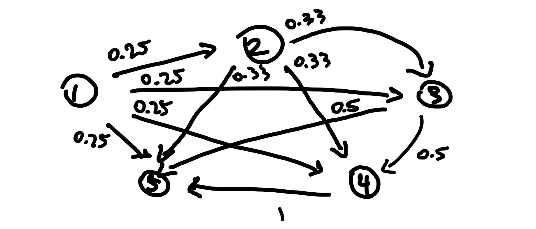
Problem 2. Smith is in jail and had $3$ dollars and can get out on bail if he has $8$ dollars. A guard agrees to make a series of bets with him, with Smith’s probability of winning $p = 0.4$ and probability of losting $p = 0.6$. Find the probability that he can leave on bail before losing all his money if he bets $1$ every time versus if he bets as much as possible each round to get to $8$ dollars but nothing more than that. Which is the optimal strategy? Solution. This problem is from Aldous’s STAT 150 class and is a spinoff of the gambler’s ruin problem. If Smith bets one dollar at a time, the Markov chain that describes his money at each state $i$ follows:

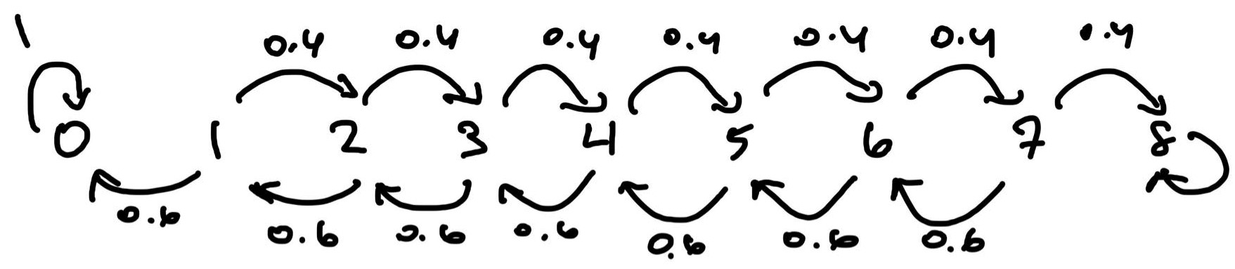
Let $p_i$, $i\in[0,8]$ be the probability that Smith’s money reaches $8$ before $0$ when starting from state $i$. Then we have

You can solve this extremely convoluted system of linear equations to find that $p_3 = 0.0964$. Alternately, the transition matrix for this Markov chain is:

Taking $P^n$ with $n$ sufficiently large gives us the steady state of this Markov chain, and $P^n_{4,9}$ gives us $p_3$ as well!

For the case that Smith bets as much as possible each round as needed to reach $8$ dollars, we have the Markov chain:

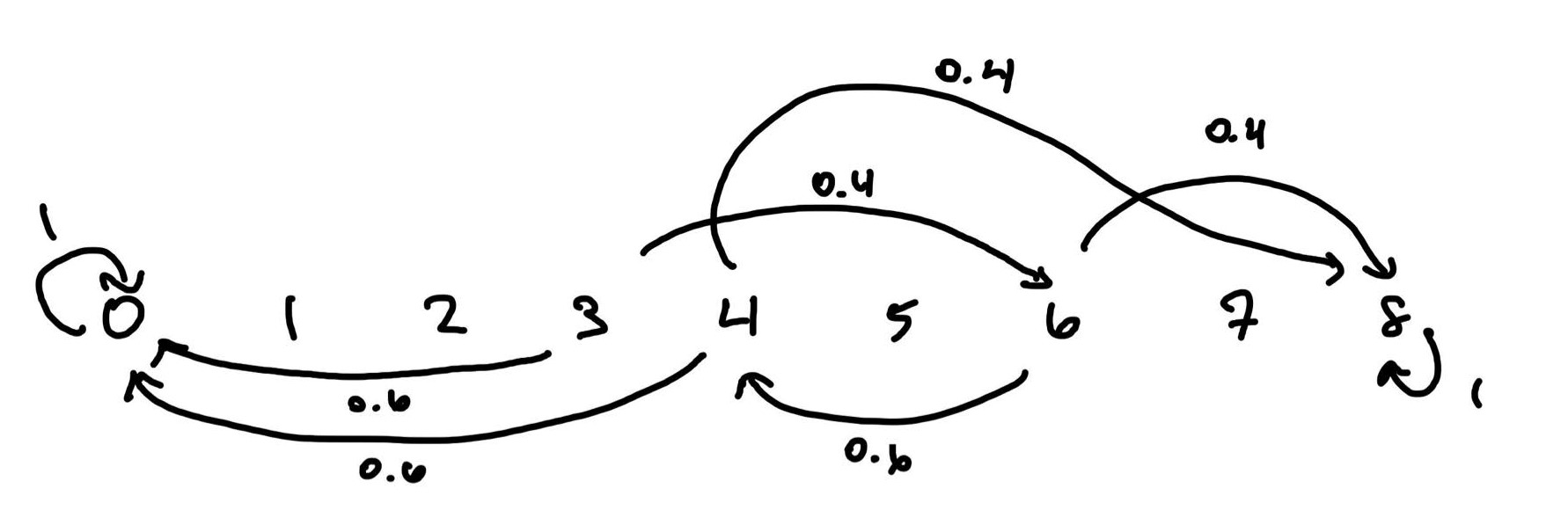
This in turn gives us the system of equations

Solving for this gives us $p_3 = 0.256$. This is considerably higher than betting one dollar each time, so Smith should choose this strategy when betting.

Problem 3. What is the expected number of tosses for a us to toss a $HTH$? Solution. This is another Markov chain problem. Note that we start all the way over whenever we roll a tails before our first heads so let’s call this state $0$. We can also account for all the other possible states: $1 = H$, $2 = HT$, and $3 = HTH$. Assuming a fair coin we have the following Markov chain:

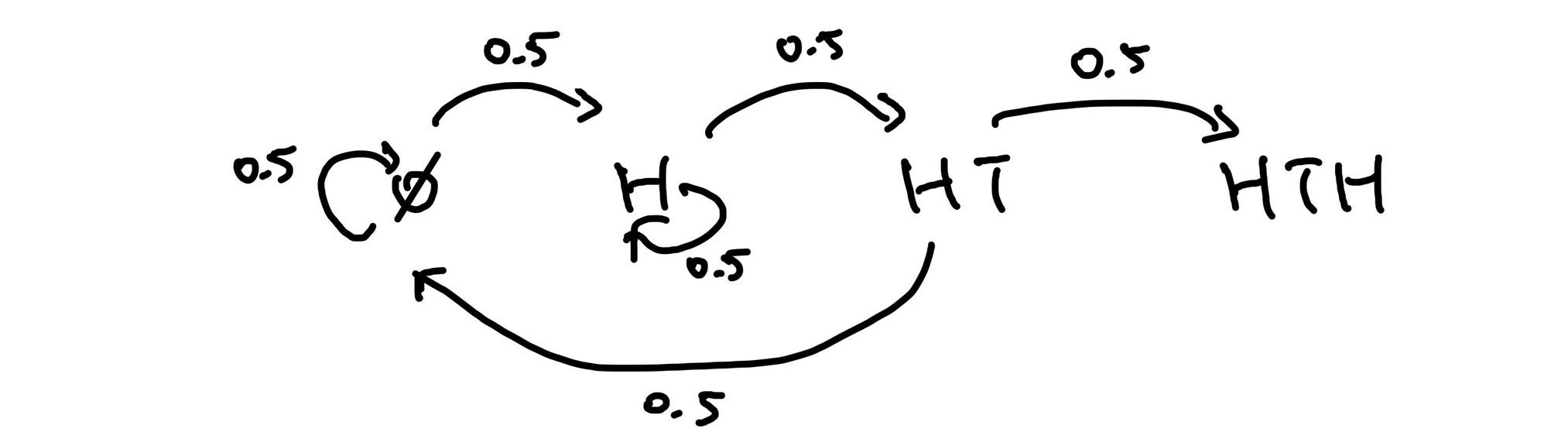
Let’s denote $\mathbb{E}[i]$ as the expected number of turns to get $HTH$ from each state $i$. Then we have the following system of linear equations:

Solving these gives $\mathbb{E}[0] = 10$ so we expect it to take 10 turns to flip our first $HTH$.

Problem 4. Players $A$ and $B$ play a marble game. Each player has a red and a blue marble in a bag and draws one marble from their bag each round. If both marbles are blue $A$ wins $\$3$ and if both are red $A$ wins $\$1$. If the two colors are different, $B$ wins $\$2$. If you can play this game 100 times, who would you play as?

Solution. Since there is an equal chance of picking marbles with different colors as picking two marbles that are the same color, the expected value of playing player $A$ versus player $B$ is the same (EV $= \$1$). Then, minimizing risk, we can calculate the variance of the payoff for each player:

$A$’s payoff has larger variance and he holds more risk so it’s advantageous to play as player $B$ when risk-averse. However, since $n$ is relatively large, the actual payoff approaches the expected payoff of playing, minimizing the risk of playing as player $A$.

Problem 5. You are trapped in a dark cave with three indistinguishable exits on the walls. One of the exits takes you 3 hours to travel and takes you outside. One of the other exits takes 1 hour to travel and the other takes 2 hours, but both drop you back in the original cave through the ceiling, which is unreachable from the floor of the cave. You have no way of marking which exits you have attempted. What is the expected time it takes for you to get outside? Solution. This is a simple EV problem. Since the doors are indistinguishable and we can’t makr our escape attempts, the probability of selecting each of the exists is identical and independent from the others. Then let $X$ be a random variable measuring the time it takes to make it out of the cave. There is $\frac{1}{3}$ chance we make it outside in time $3$, $\frac{1}{3}$ chance we waste an hour and end up back in the cave, and $\frac{1}{3}$ chance we waste two hours and end up back in the cave. Then,

Solving this equation gives $\mathbb{E}[X] = 6$ so we expect to spent $6$ hours attempting to escape before we’re finally outside.

Day Nine: June 30

For today’s problems I took a step back and reviewed some general problems and conditional probability.

Problem 1. A deck of cards has 3 Red and 3 Blue cards. At each stage, a card is selected at random. If it is Red, it is removed from the deck. If it is Blue then the card is not removed and we move to the next stage. Find the average number of steps till the process ends. Solution. Note that the proces ends when there are no red cards left. To get started, I’ll draw the Markov chain for this problem:

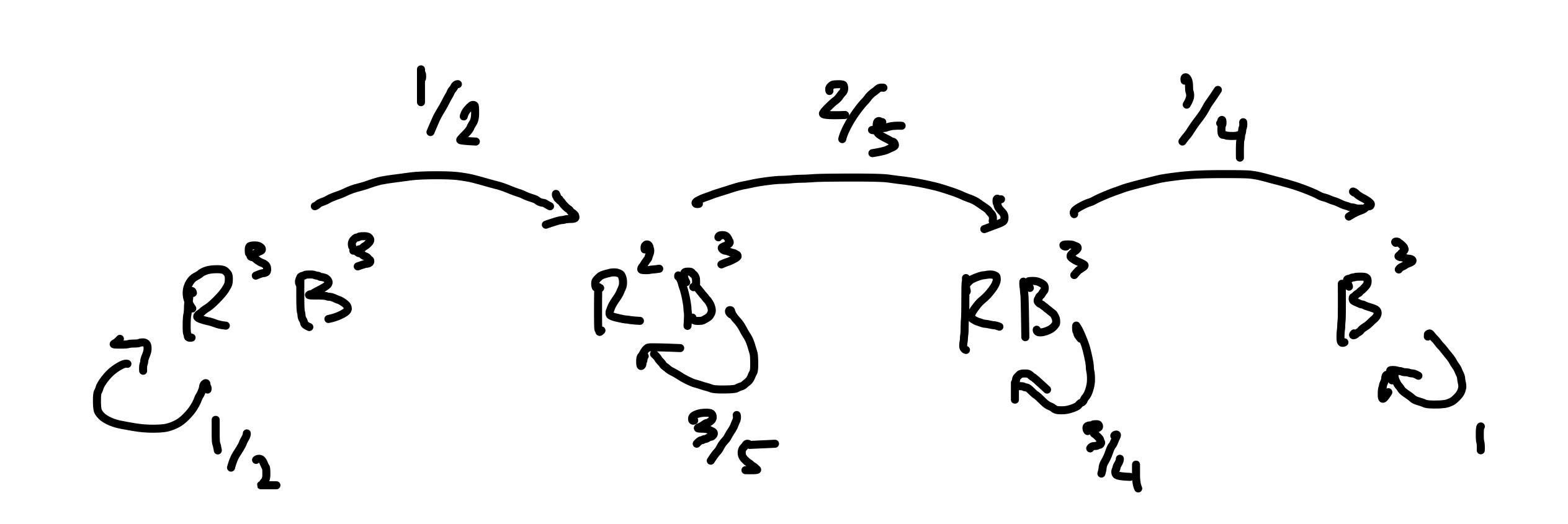
Now let’s index the states: State $0 = R^3B^3$, State $1 = R^2B^3$, State $2 = RB^3$, State $3 = B^3$. Let $\mathbb{E}[i]$ denote the expected time until the process ends. Then we have the following equations:

Solving this system gives $\mathbb{E}[0] = 8.5$.

Problem 2. A process moves on the integers 1, 2, 3, 4, and 5. It starts at 1 and, on each successive step, moves to an integer greater than its present position, moving with equal probability to each of the remaining larger integers. State five is an absorbing state. Find the expected number of steps to reach state five. Solution. The Markov chain for this problem is

This gives us the transition matrix

We’re interested in finding the expected number of steps to reach state five from state one so let $\mathbb{E}[i]$ denote the expected number of steps to reach step $5$ from step $i$. Then we have the equations

Solving this system of linear equations gives us the set of expected steps from each state $\{\mathbb{E}[1], \mathbb{E}[2], \mathbb{E}[3], \mathbb{E}[4], \mathbb{E}[5]\} = \{\frac{25}{12}, \frac{11}{6},\tfrac{3}{2}, 1, 0\}$ so we expect about $2.0833$ steps to reach $5$.

Problem 3. An unfair coin has probability $p$ of tossing heads and $q = 1-p$ of tossing tails. How do you make this coin fair? Solution. Note that $p_H = p$ and $p_T = p$. The only way for us to make the coin fair is to somehow combine the $H,T$ outcomes as rolling consecutive heads vs tails has different probability of success. Note that $HT$ is rolled with a probability of $pq$ and $TH$ is rolled with a probability of $qp$ (note these are equal). Also $HH$ has $p = p^2$ and $TT$ has $p = q^2$. We can modify the typical rules of coin flipping in in the following way to make it fair: Let heads be tossing an $HT$ and tails be tossing $TH$, which both have equal probability and is fair. Then, to account for the remaining two possible outcomes, we just start over when we get $HH$ or $TT$, which gives us an automatic reset when we toss two of the same face. Technically, $HHT$ would be rolling a $HT$, but note that $P(HHT) = p^2q \neq q^2p = P(TTH)$ so we can’t simply take the first occurance of $HT$ or $TH$ as a fair outcome is not guaranteed.

Problem 4. This is a variation of the gambler’s ruin problem. You have $9$ and want to reach $10$. Your probability of success is $p = 0.4$ and failure is $q=0.6$. You may only place bets in multiples of $10p$. How would you maximize the probability of reaching $10$? Solution. I would bet $\$4$ each time I play. Note that from $\$9$ we can bet either $4$ or $8$. We have $p= 0.4$ of reaching $\$10$ from each of these bets, but $0.6$ chance of reaching $\$1$ if we bet $8$ dollars and $q$ chance of reaching $\$5$ if we bet $4$ dollars. Once we reach $1$, we can no longer bet as all of our bets must be a multiple of $4$. Then, if we bet $\$8$, we have a total of probability $0.4$ to reach our goal. If we bet $\$4$, then we have probability $0.4$ of getting to $\$10$ the first round. If this doesnt happen and we lose the first bet instead, then we’re at $\$5$ and we have the opportunity to go down to $\$1$ (probability $0.4$) in which we’re done and can’t bet anymore or go back up of $\$9$ and play over our original scenario over again. Clearly, betting $\$4$ per round is optimal as we have probability $0.4$ of winning the first round (matching the probability of winning when betting $\$8$) and there also is some additional probability $p_0 >0$ that we can reach $\$10$ in later rounds.

Problem 5. Two players, $A$ and $B$, toss a fair coin in that order. The sequence of heads and tails is recorded. If there is a $HT$ sequence in the rolls, then whoever rolled the tails wins and the game ends. What is the probability that $A$ wins? Solution. Let $P(A)$ and $P(B)$ denote the probabilities that $A$ and $B$ win respectively. Note that $P(B) = 1 - P(A)$. This next part is pretty cool—we can condition $P(A)$ on $A$’s first coin toss, with has probability $0.5$ to roll $H$ and probability $0.5$ to roll $T$. Then we have $P(A) = \tfrac{1}{2}P(A \, | \, H) + \frac{1}{2}P(A \, | \, T)$. If $A$ tosses heads, then $B$ essentially becomes the first to toss and so $P(A , |, T) = P(B) = 1-P(A)$. If $A$ tosses heads however, we can then condition the probability further on $B$’s first toss. $B$ has probability $0.5$ of rollng $T$, in which $A$ loses, and probability $0.5$ of tossing $H$, which essentially brings us to the scenario that $B$ is the first person to toss an $H$ so $A$ would have probability $1-P(A \, | \, H)$ of winning. Then we have

We can then plug this back into the original expresion to find that $P(A) = \frac{4}{9}$.

Day Ten: July 1

Come back later for the rest of today’s problems! My friend recommended me take a look at Fifty Challenging Problems in Probability, and I’m taking a couple of todays problems from here.

Problem 1. You play a game with an urn that contains $75$ clue balls $25$ red balls and $1$ yellow ball. For each red ball you draw you gain a dollar and if you draw the yellow ball you lose everything and the game ends. What is your strategy for this game given that you can decide to stop or redraw after each turn? Solution. Note the payoff for each blue ball draw is $0$ and the payoff for the yellow ball is $-r$ where $r$ is the number of red ball already drawn. If we let $b$ be the number of blue balls already drawn, we can derive the marginal expected value (not sure if this is a term):

Our marginal $EV$ should be greater than $0$ for us to keep playing. Then, setting the numerator to $0$ and solving gives us $r= \frac{25}{2}$. This is the number of balls that have already been drawn, so after drawing $12$ balls our $EV$ is still positive so we’ll draw a $13$th one. Then we draw $13$ balls and call it a day (of course this will sometimes be cut short if we draw a yellow ball before then).

Problem 2. A drawer contains red socks and and black socks. When two socks are chose at random, the probability that both are red is $\frac{1}{2}$. How small can the number of socks in the drawer be? Solution. Let $r$ and $b$ denote the number of red and black socks respecively. Since we are selecting socks without replacement, we have

Then,

Note that $b\neq 0$ since $P(r \, | \, b = 0) = 1$. So if we choose $b= 1$ and plug it into the quadratic equation to solve for $r$, in which case we get $r = 3$. Then, the minimum number of socks in the drawer is $\$4$.

Problem 3. Mr. Brown always bets a dollar on the number $13$ at roulette agains the advice of his friend. To help cure Mr. Brown of playing roulette , his friend bets Brown $\$20$ at even money that Mr. Brown will be behind at the end of $36$ plays. How is the cure working? Mr. Brown is piad $\$35$ of his bet amount in roulette when his number comes up and roulette has $38$ numbers to bet on. Solution. In order to go even in $36$ rounds, Mr. Brown needs only win one turn. So he’ll be behind if he loses all $36$ turns, which has probability $(\frac{37}{38})^36 = 0.383$, which is the probability that he loses his bet with his friend. Note also that his ev after 36 turns is

Then Mr. Brown’s EV of betting with his friend is

So this cure doesn’t seem to be working too well. Mr. Brown’s EV of eahc cycle of $36$ turns is $\$2.79$ whenever he makes the $\$20$ bet with his friend.

Problem 4. We throw three dice one by one. What is the probability that we roll three nunbers in strictly increasing order? Solution. Note that in order for the three numbers to be in strictly increasing order, they have to be unique. Then $P(\text{unique and strictly increasing}) = P(\text{unique})$. We have probability $\frac{6}{6} \cdot \frac{5}{6} \cdot \frac{4}{6} = \frac{5}{9}$. When conditioned on us rolling three numbers, the probability of rolling strictly increasing numbers is simply based on how we want them arranged. There is only one correct arragement, but there are $6$ ways to choose how to arrange the three numbers, so we have $P(\text{stringtly increasing} \, | \, \text{unique}) = \frac{1}{6}$. Then we have

Then we have probability $0.093$ of rolling such an outcome.

Problem 5. The game of craps, played with two dice, is one of America’s fastest and most popular gambling games. These are the rules: we throw two dice. If we roll $7$ or $11$ on the first throw, we win immediately and if we roll $2, 3$ or $12$ we lose immediatly. And other throw is called a “point”. If the first toss is a point, then we keep rolling until we roll our point, or roll a $7$ and lose. Wht is the probability of winning? I thought this was a Markov chain problem at first but a closer look made me realize it was just a bit of conditional probability. Note how I got the numbers: there are $36$ outcomes for two dice. There is one way for me to roll a $2$, on way to roll a $12$, abd $2$ ways to roll a $3$. Then the probabiity of losing the first round is $\frac{1 + 1+ 2}{36} = \frac{1}{9}$. Additionally, there are $6$ ways to roll a $7$ and $2$ ways to roll an $11$ so our probability of winning the first round is $\frac{2}{9}$ and there is a $\frac{2}{3}$ chance of rolling a point. Now, we just need to find the probability of winning conditioned on rolling a point and adding that to the probability of winning the first round to arrive at the total probability of winning. Note that there is probability $\frac{1}{12}$ that we roll $4$ or $10$, $\frac{1}{9}$ that we roll a $5$ or a $9$, and $\frac{5}{36}$ of rolling a $6$ or an $8$.

Note that in the event that we roll a point in our first round, we need only consider the probabilities of rerolling the point (to win) or a $7$ (to lose) as rolling a nonpoint/seven will bring us back to our original scenario of wanting to roll the point. Then, there is probability $\frac{3}{3 + 6}$ of rolling a $4$ or $10$, $\frac{4}{6}$ of rolling of a $5$ or $9$, $\frac{5}{5+6}$ of rolling a $6$ or an $8$ (these can all be calculated by the number of ways to roll the point vs. the $7$). Then, the probability of winning conditional on rolling a point the first turn is

Adding this to $\frac{2}{9}$, which is our probability of winning round $1$, we have a total probability of winning $p = 0.493$, which is relatively fair for a casino game.

Day Eleven: July 2

Dynamic programming is also relatively fair game at some trading firms so I’ve included some dp questions for future problems.

Problem 1. A basketball player is taking $100$ free throws. She scores one point if the ball passes through the hoop and zero point if she misses. She has scored on her first throw and missed on her second. For each of the following throw the probability of her scoring is the fraction of throws she has made so far. For example, if she has scored $23$ points after the $40^\text{th}$ throw, the probability that she will score in the $41^\text{th}$ throw is $23/40$. After $100$ throws (including the first and the second), what is the probability that she scores exactly $50$ baskets? Solution. This is another problem from A Practical Guide. I approached this problem with the mindset of Markov chains at first but then I realized that I could build it up iductively with conditional probability. Let’s define $(n,k)$ to be the event that the player scores $k$ baskets after $n$ shots and $p_{n,k} = P((n,k))$. Since we make the first shot and miss the second, the third shot has success probability $\frac{1}{2}$ ($p_{3,1} = \frac{1}{2} = p_{3,2})$. For $n=4$, we can condition it on $(3,1)$ and $(3,2)$ having taken place. Then,

$p_{4,1} = P((4,1)\, | \, P(3,1)) + P((4,1)\, | \, P(3,2)) = \frac{2}{3}\cdot \frac{1}{2} + 0 \cdot \frac{1}{2} = \frac{1}{3}$
$p_{4,2} = P((4,2)\, | \, P(3,1)) + P((4,2)\, | \, P(3,2)) = \frac{1}{3} \cdot \frac{1}{2} + \frac{1}{3} \cdot \frac{1}{2} = \frac{1}{3}$
$p_{4,3} = P((4,3)\, | \, P(3,1)) + P((4,3)\, | \, P(3,2)) = 0 \cdot \frac{1}{2} + \frac{1}{2} \cdot \frac{2}{3} = \frac{1}{3}$

The pattern seems to be emerging that $p_{n,k} = \frac{1}{n-1}$ for $k \in [1, n]$ regardless of what $k$ is (obviously $k < n$ since we have missed the second shot), which we can prove inductively.
Base Case: $p_3$ is our base case
Inductive Step: Suppose that $P_{n,k} = \frac{1}{n}$ holds for all $k \in [1, n]$. Then for $n+1$:

Then we have probability $\frac{1}{99}$ of making exactly $50$ shots out of $100$.

Problem 2. Dynamic Programming: Given two arrays of numbers, find the length of the largest subsequence present in both arrays. For example the length of largest subsequence present in $[1,2,3,4]$ and $[2,3,5,7]$ is $2$. Solution. Our goal is to build a method that returns the largest common subsequence (lcs). Let’s look at the brute force solution: we can approach the problem by finding each of the substrings in one of the arrays and seeing if it is present in the second array. There are $\binom{n}{k}$ combinations for substrings of length $k$ given an array of length $n$. Then we have $\binom{n}{1} + \binom{n}{2} + \cdots + \binom{n}{n} = 2^n$ operations for our brute force solution, indicating $O(2^n)$ time. Now let’s approach it with dynamic programming: assuming our first array has length $m$ and our second array has length $n$, we can build an $m\times n$ matrix in which the $(i,j)$ entry holds the size of largest common multiple of $\text{array1}[0, 1, \dots i]$ and $\text{array2}[0, 1, \dots j]$.Then we have the following solution in C++:

int largestCommonSubsequence(int *array1, int *array2){
	int m = array1.size();
	int n = array2.size();
	int lcs[m+1][n+1]; // our "matrix"

	// constructs m by n matrix of lcs's using dp
	for(int i = 0; i < m; i++){
		for(int j = 0; j < n; j++){
			if(i == 0 || j == 0){
				lcs[i][j] = 0;
			} else if (array1[i-1]= array2[j-1]){
				lcs[i][j] = lcs[i - 1][j - 1] + 1;
			} else{
				lcs[i][j] = max(lcs[i-1][j], lcs[i][j-1]);
			}
		}
		return lcs[m][n];
	}
}

Walking through the for loop: when either $i$ or $j$ is $0$, at least one of the two subarrays we’re looking at are empty. Then, the lcs is just $0$. Otherwise, if the previous number we looked at in the first array is the same as the previous number we looked at in the second array, then we simply need to add one to the value of our previous $(i,j)$ entry since we’ve increased the common subseqeunce by one number. Finally, if neither of these are the case, the lcs of the current $i,j$ matrix is the same as the max of the previous $i-1 \times j$ or $i \times j-1$ matrix. This solution has an $O(mn)$ time, where $m$ and $n$ are the lengths of the two arrays.

Problem 3. $500$ ants are randomly put on a $1$-foot string (independent uniform distribution for each ant between $0$ and $1$ ). Each ant randomly moves toward one end of the string (equal probability to the left or right) at constant speed of $1$ foot/minute until it falls off at one end of the string. Also assume that the size of the ant is infinitely small. When two ants collide head-on, they both immediately change directions and keep on moving at $1$ foot/min. What is the expected time for all ants to fall off the string? Solution. This problem is relatively simple when you start thinking about it. The most troublesome part seems to be the collision as each collision complicates the process and each any can collide with another at any time. Interesting collisions don’t seem to be relevant to solving this question. When an ant moving to the right collides with an ant moving to the left, the result is the two ants switching directions, but there is still one ant moving left and one ant moving right (at the same speed as well). So its’ as if collisions don’t really take place. Then, the expected time is just the max time for an ant to move across the string given a uniform distribution. This is identical to asking what the expected value of the maximum of $500$ i.i.d random variables with uniform distribution on $[0,1]$, aka an order statistic problem. Lets find the CDF of $X_{500}$, the maximum of the independently distributed ants.

Then, we can find the PDF by differentiating to get $p_X(x)= 500x^{499}$. The expected value of the max of the $500$ i.i.d random variables is

There is an alternate solution to this problem on the Berkeley EECS 126 site, where it’s listed as a test review problem.

Problem 4. In a common carnival game a player tosses a penny from a distance of about five feet onto the surface of a table ruled in $1$-inch squares. If the penny (diameter $\frac{3}{4}$ inch) falls entirely inside a square, the player received five cents but does not get his penny back and he loses his penny otherwise. If the penny lands on the table, what is the expected payoff of the game. Solution. We’re given that that the penny lands on the table so we know that the penny will fall on a square. Then we only need to find the regions where our penny can land on for it to be fully encapsulated. I’ve drawn two diagrams to model two different appraoches to this problem. We cant first visualize the penny landing on any four-square unit since any four adjacent squares are guaranteed to fully encompass a penny. Then, the part of the penny that associates with each corner must be squeezed into one of the four $\frac{1}{4} \cdot \frac{1}{4}$ squares, which has a total area of $\frac{1}{4}$ and probability $\frac{1}{16}$ of being landed on.

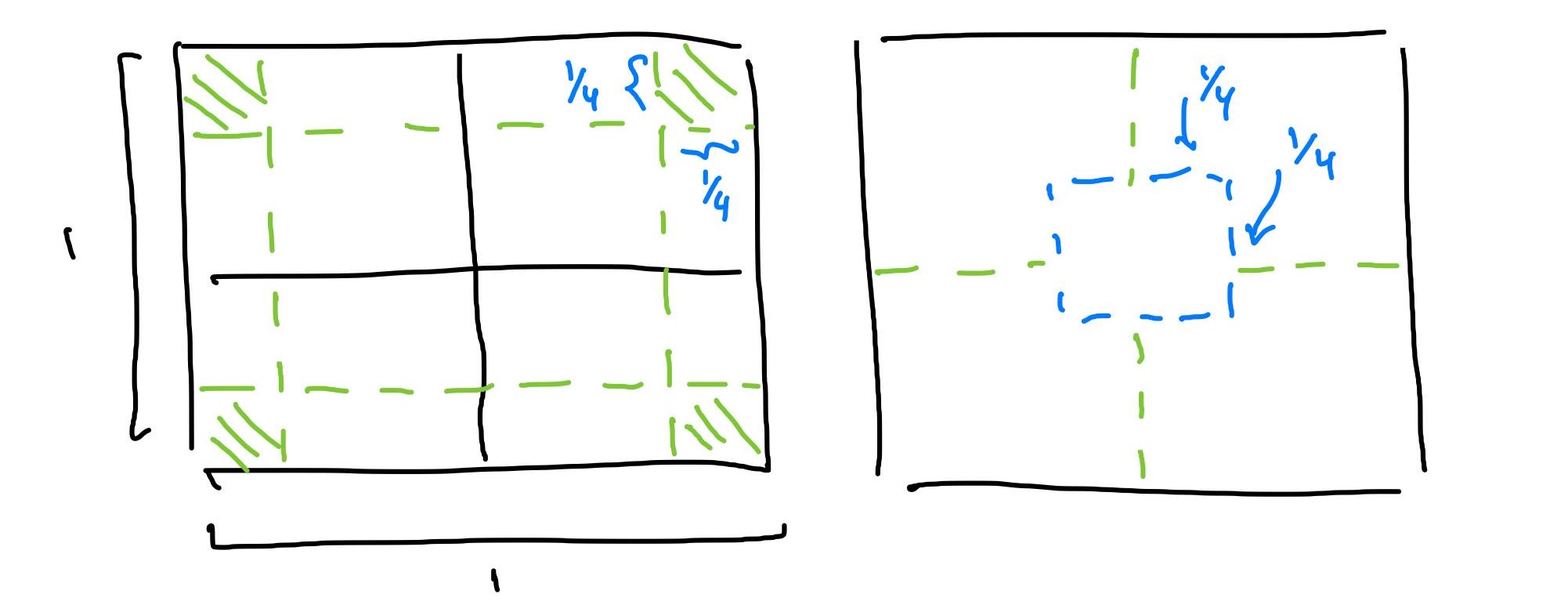
Regarding the second visualization, this is much more accurate to the possible outcomes of the penny toss since we cannot have an edge of the penny touch a specific corner of the square. Then, we can visualize the locations that the center of the penny must reside in. The radius of the penny is $\frac{3}{8}$ so the center of the penny must reside at least $\frac{3}{8}$ inch from each side of the square, giving a smaller square of potential center point wuth area $\frac{1}{16}$. Then, the expected value of the game is $-1 \cdot \frac{15}{16} + 4 \cdot \frac{1}{16} = \frac{-11}{16}$.

Problem 5. Eight eligible men and seven women happen randomly to have purchased single seats in a $15$ seat row of a theater. On average, how many pairds of adjacent seats, are ticketed for marriageable couples? Solution. The book that this problem is from is a bit old so the wording is a bit old-fashioned. Essentially we’re looking to find the average number of potential male-female couples who sit next to one another. The best case and worst case scenario follow

In order to build a marriageable couple we need to have $\text{MW}$ or $\text{WM}$, or unlike adjacent seatings. If they are unlike, then we have $1$ marriageable couple and if not then we have $0$. The probability of a marriageable couple in the first two seats is $2 \cdot\frac{8}{15} \cdot \frac{7}{14}$. Note that $\frac{8}{15}$ is also the expected number of marriageable couples in the first two seats. Our sam calculation can applies to any adjacent pair so we can get the average number of marriageable adjacent pairs by taking the number of adjacent pairs and multiplying by the expected value of each adjacent pair being marriageable: $14 \cdot \frac{8}{15} = \frac{112}{15} \approx 7.47$. Then the expected number of marriageable couples is just under half of the people present.

Moving on to a more general case, when we can $b$ elements of one type and $m$ of another randomly arranged in a line, the expected number of unlike adjacent elements is

which can be shown easily by going through the same process we used for our specific case.

Day Twelve: July 3

Come back later for today’s problems!

Problem 1. Two players bet on the number of rolls of the total of two standard six faced dice. Player $A$ bets tha a sum of $12$ will occur first and player $B$ bets that two consecutive $7$’s will be rolled before that. What is the probability that $A$ will win? Solution. This question can be solved either through conditional probability or a Markov chain approach. I’ve opted for a Markov chain since it’s much more straightforward and easily illustrated. Below is the Markov diagram for this problem. I’ve chosen to denote $\empty$ the event of rolling for the first time. Since every time we roll something other than a $7$ or a $12$ we essentially reset, each state gives us a certain probability of returning to our original state. It’s worth noting that after rolling the first $7$ there is still a nontrivial probability for $B$ to win as $12$ can still be rolled in the next round.

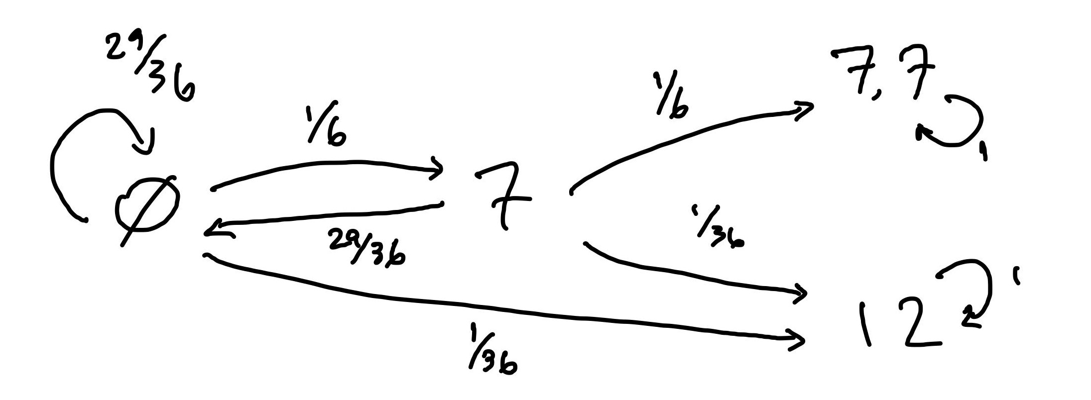
Then we have the following system of equations to solve:

Noting that $p_{7,7} = 0$ and $p_{12} = 1$, solving gives us that $p_\empty = \frac{7}{13}$. Then, player $A$ is slightly favored to win over player $B$ in their bet.

Problem 2. There are 51 ants on a square with side length of 1. If you have a glass with a radius of 1/7, can you put your glass at a position on the square to guarantee that the glass encompasses at least 3 ants? Solution. We can do this by creating $25$ sub-squares and using the pidgeonhole principle to conclude that ones of these sub-squares must have at least $3$ ants. In creating these $25$ sub-squares, we want them to cover the entirety of the original $1\times 1$ square so each of these smaller squares will have a $\frac{1}{5}$ side length. Note that a sub-square with side length $\frac{1}{5}$ has diagonal length $\sqrt{2}\frac{1}{5} \approx 0.282$. Meanwhile, the radius $\frac{1}{7}$ glass cup has a diameter of $\frac{2}{7} \approx 0.285$, so any sub-square can be inscribed within the glass. Then, we simply need to choose the sub-square with the most ants and place our glass carefully to cover at least three ants.

Problem 3. The probability you’ll see a falling star in the sky over the course of one hour is 0.44. What’s the probability you’ll see one over half an hour? Solution. This is a past Citadel interview question that I’ve seen variants of at other companies. We can assume that each half hour is independent from the other regarding falling star appearances. Then, the probability of not seeing a shooting star in either half-hour intervals is $0.56$. Let $p$ be the probability that we see a shooting star in a thirty minute interval. Then we have

Solving gives us $p \approx 0.25$. This question is meant to be solved mentally so I didn’t include and pen or paper for it. For taking the square root of $0.56$, I did a linear approximation based off of $\sqrt{0.49}$ and $\sqrt{0.64}$.

Problem 4. You are given two ropes that when lit burn in one hour. Which one of the following time periods CANNOT be measured with your ropes? a) 50 min b) 30 min c) 25 min d) 35 min. Solution. The only time period I can’t think of a solution to is $50$ min. The key to this problem is realizing that we can burn the rope wherever we want. It’s easy to finding $30$ minutes by burning a single rope on both ends. We can burn $35$ by first measuring $30$ minutes. Then, we measure $5$ additional minutes by burning the second rope on both ends and $5$ additional times in the middle. This process will create two ropes, all of which burn on both of their ends. If any of these ropes burn out fully, all we need to do is light one of the other $5$ ropes in the middle. Keep doing this proccess and you’ll have an additional $5$ minutes measured. To measure $25$ minutes, we can burn one of the ropes on both ends and once in the middle. If one of the two ropes formed by the burning burns out, then light the other sub-rope in the middle, making sure the rope is still burning in $4$ places. This ensures that the first rope will finish burning in $10$ minutes. Then, we need only light the second rope on both ends and two times in the middle. This ensures the second rope burns at $6$ places, and so we’ll measure $10$ additional minutes that way.

Problem 5. You have three cards, each labeled $n$, $n+1$, $n+2$, and you don’t know $n$. All cards start facing down so you can’t see them. You flip one card. If you choose to “stay”, you get that card’s value. If you don’t “stay”, then you flip another card. Again, choose to “stay” (and keep the 2nd card’s value) or flip the final card and keep the final card’s value. Design the optimal strategy to maximize the value of the card that you choose and find the expectation of that value. Solution. Note that your expected value will be at least $n$. Making our decision on draw $1$ ensures we have no information and making our decision of draw $3$ presents us with no choice. Then it makes sense for us to make our decision on round $2$. Since we have the ability to draw once again after round $2$, our decision is simply to take what we drew or draw again. I will refer to each draw $i$ as $d_i$. Then, if
$d_2 - d_1 = -2:$ we have the sequence $n+2, n, n+1$ so we choose to draw again for ev $n+1$
$d_2 - d_1 = 2:$ we have the sequence $n, n+2, n+1$ so we stay for ev $n+2$
$d_2 - d_1 = 1:$ we either go up $1$ ($n,n+1, n+2$) or down $2$ ($n+1, n+2, n$) so we choose to stay for ev $n + 1.5$ $d_2 - d_1 = -1:$ we either go up $2$ ($n+1, n, n+2$) or down $1$ ($n+2, n+1, n$) so we choose to draw again for ev $n+1$ Using this strategy, we combine our total expected value:

My optimal strategy is to draw the first two cards and determine whether to draw again with the thought process above with expected value $n + \frac{4}{3}$. Putting it more simply, if the second draw is higher than the first, then stay, and if not, then draw again.

Week Two Review:

This week I focused on working through more of A Practical Guide, and starting to pull general probability question from resources. i’ve done a bit of market-making practice behind the scenes and am still figuring out the best way of going about that. I didn’t get to review as many topics as I had hoped to and next week I hope to work on some more programming/staticstics questions as recruiting season begins.

Here are this week’s list of resources:

• A Practical Guide to Quantitative Finance Interviews (Ch 2, 4)
• Fifty Challenging Problems in Probability
• eFinancialCareers Past Interview Questions
• Confidence Intervals
• MIT Quant Finance Presentation
• Citadel Glassdoor Questions